DenMune: A density-peak clustering algorithm
DenMune a clustering algorithm that can find clusters of arbitrary size, shapes and densities in two-dimensions. Higher dimensions are first reduced to 2-D using the t-sne. The algorithm relies on a single parameter K (the number of nearest neighbors). The results show the superiority of the algorithm. Enjoy the simplicity but the power of DenMune.

![]()
![]()


Based on the paper
Paper |
Journal |
|---|---|
Mohamed Abbas, Adel El-Zoghabi, Amin Ahoukry |
|
DenMune: Density peak based clustering using mutual nearest neighbors |
|
In: Journal of Pattern Recognition, Elsevier, |
|
volume 109, number 107589, January 2021 |
|
Documentation:
Documentation, including tutorials, are available on https://denmune.readthedocs.io
Watch it in action
This 30 seconds will tell you how a density-baased algorithm, DenMune propagates:
![]()

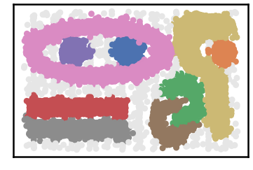
When less means more
Most calssic clustering algorithms fail in detecting complex where clusters are of different size, shape, density, and being exist in noisy data. Recently, a density-based algorithm named DenMune showed great ability in detecting complex shapes even in noisy data. it can detect number of clusters automatically, detect both pre-identified-noise and post-identified-noise automatically and removing them.
It can achieve accuracy reach 100% in most classic pattern problems, achieve 97% in MNIST dataset. A great advantage of this algorithm is being single-parameter algorithm. All you need is to set number of k-nearest neighbor and the algorithm will care about the rest. Being Non-senstive to changes in k, make it robust and stable.
Keep in mind, the algorithm reduce any N-D dataset to only 2-D dataset initially, so it is a good benefit of this algorithm is being always to plot your data and explore it which make this algorithm a good candidate for data exploration. Finally, the algorithm comes with neat package for visualizing data, validating it and analyze the whole clustering process.
Installation and Usage
Install It:
Simply install DenMune clustering algorithm using pip command from the official Python repository
From the shell run the command
pip install denmune
From jupyter notebook cell run the command
!pip install denmune
Import It:
Once DenMune is installed, you just need to import it
from denmune import DenMune
Note
Please note that first denmune (the package) is in small letters, while DenMune (the class itself) has D and M in capital case while other letters are small.
Loading data
There are four possible cases of data:
only train data without labels
only labeld train data
labeled train data in addition to test data without labels
labeled train data in addition to labeled test data
#=============================================
# First scenario: train data without labels
# ============================================

data_path = 'datasets/denmune/chameleon/'
dataset = "t7.10k.csv"
data_file = data_path + dataset

# train data without labels
X_train = pd.read_csv(data_file, sep=',', header=None)

knn = 39 # k-nearest neighbor, the only parameter required by the algorithm

dm = DenMune(train_data=X_train, k_nearest=knn)
labels, validity = dm.fit_predict(show_analyzer=False, show_noise=True)
This is an intutive dataset which has no groundtruth provided
#=============================================
# Second scenario: train data with labels
# ============================================

data_path = 'datasets/denmune/shapes/'
dataset = "aggregation.csv"
data_file = data_path + dataset

# train data with labels
X_train = pd.read_csv(data_file, sep=',', header=None)
y_train = X_train.iloc[:, -1]
X_train = X_train.drop(X_train.columns[-1], axis=1)

knn = 6 # k-nearest neighbor, the only parameter required by the algorithm

dm = DenMune(train_data=X_train, train_truth= y_train, k_nearest=knn)
labels, validity = dm.fit_predict(show_analyzer=False, show_noise=True)
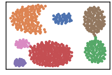
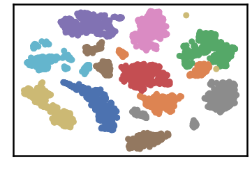
Datset groundtruth

Datset as detected by DenMune at k=6
#=================================================================
# Third scenario: train data with labels in addition to test data
# ================================================================

data_path = 'datasets/denmune/pendigits/'
file_2d = data_path + 'pendigits-2d.csv'

# train data with labels
X_train = pd.read_csv(data_path + 'train.csv', sep=',', header=None)
y_train = X_train.iloc[:, -1]
X_train = X_train.drop(X_train.columns[-1], axis=1)

# test data without labels
X_test = pd.read_csv(data_path + 'test.csv', sep=',', header=None)
X_test = X_test.drop(X_test.columns[-1], axis=1)

knn = 50 # k-nearest neighbor, the only parameter required by the algorithm

dm = DenMune(train_data=X_train, train_truth= y_train,
             test_data= X_test,
             k_nearest=knn)
labels, validity = dm.fit_predict(show_analyzer=True, show_noise=True)
dataset groundtruth
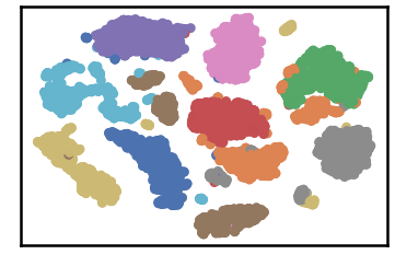
dataset as detected by DenMune at k=50
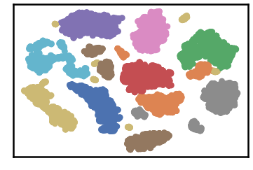
test data as predicted by DenMune on training the dataset at k=50
Algorithm’s Parameters
Parameters used within the initialization of the DenMune class
def __init__ (self,
                  train_data=None, test_data=None,
                  train_truth=None, test_truth=None,
                  file_2d ='_temp_2d', k_nearest=10,
                  rgn_tsne=False, prop_step=0,
                  ):
train_data:
data used for training the algorithm
default: None. It should be provided by the use, otherwise an error will riase.
train_truth:
labels of training data
default: None
test_data:
data used for testing the algorithm
test_truth:
labels of testing data
default: None
k_nearest:
number of nearest neighbor
default: 10. It should be provided by the user.
rgn_tsn:
when set to True: It will regenerate the reduced 2-D version of the N-D dataset each time the algorithm run.
when set to False: It will generate the reduced 2-D version of the N-D dataset first time only, then will reuse the saved exist file
default: True
file_2d: name (include location) of file used save/load the reduced 2-d version
if empty: the algorithm will create temporary file named ‘_temp_2d’
default: _temp_2d
prop_step:
size of increment used in showing the clustering propagation.
leave this parameter set to 0, the default value, unless you are willing intentionally to enter the propagation mode.
default: 0
Parameters used within the fit_predict function:
def fit_predict(self,
                   validate=True,
                   show_plots=True,
                   show_noise=True,
                   show_analyzer=True
                   ):
validate:
validate data on/off according to five measures integrated with DenMUne (Accuracy. F1-score, NMI index, AMI index, ARI index)
default: True
show_plots:
show/hide plotting of data
default: True
show_noise:
show/hide noise and outlier
default: True
show_analyzer:
show/hide the analyzer
default: True
Features
The Analyzer
The algorithm provide an intutive tool called analyzer, once called it will provide you with in-depth analysis on how your clustering results perform.
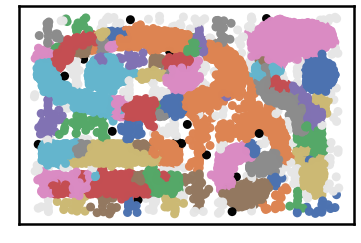
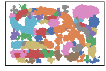
Noise Detection
DenMune detects noise and outlier automatically, no need to any further work from your side.
It plots pre-identified noise in black
It plots post-identified noise in light grey
You can set show_noise parameter to False.
# let us show noise

m = DenMune(train_data=X_train, k_nearest=knn)
labels, validity = dm.fit_predict(show_noise=True)
# let us show clean data by removing noise

m = DenMune(train_data=X_train, k_nearest=knn)
labels, validity = dm.fit_predict(show_noise=False)
noisy data |
clean data |
|---|---|
|
|
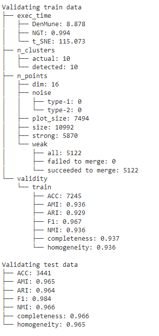
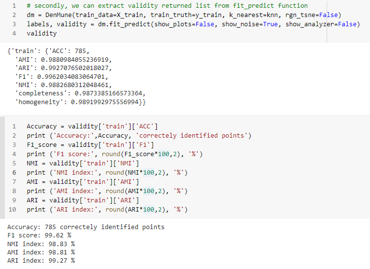
Validatation
You can get your validation results using 3 methods
by showing the Analyzer
extract values from the validity returned list from fit_predict function
extract values from the Analyzer dictionary
There are five validity measures built-in the algorithm, which are:
ACC, Accuracy
F1 score
NMI index (Normalized Mutual Information)
AMI index (Adjusted Mutual Information)
ARI index (Adjusted Rand Index)
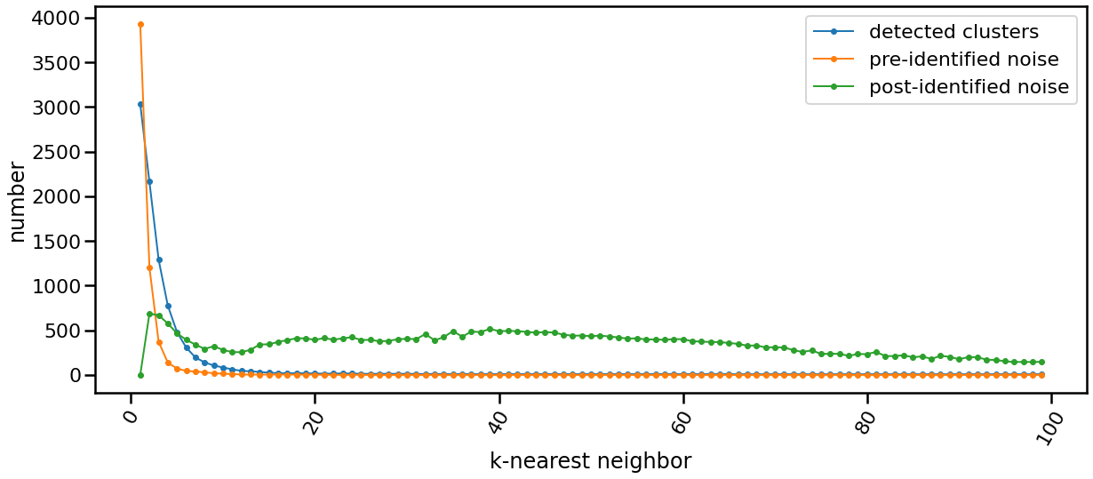
K-nearest Evolution
The following chart shows the evolution of pre and post identified noise in correspondence to increase of number of knn. Also, detected number of clusters is analyzed in the same chart in relation with both types of identified noise.
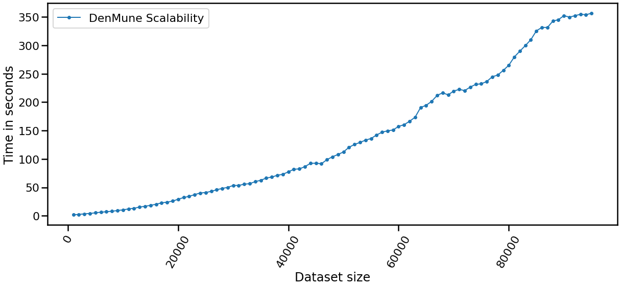
The Scalability
data size |
time |
|---|---|
data size: 5000 |
time: 2.3139 seconds |
data size: 10000 |
time: 5.8752 seconds |
data size: 15000 |
time: 12.4535 seconds |
data size: 20000 |
time: 18.8466 seconds |
data size: 25000 |
time: 28.992 seconds |
data size: 30000 |
time: 39.3166 seconds |
data size: 35000 |
time: 39.4842 seconds |
data size: 40000 |
time: 63.7649 seconds |
data size: 45000 |
time: 73.6828 seconds |
data size: 50000 |
time: 86.9194 seconds |
data size: 55000 |
time: 90.1077 seconds |
data size: 60000 |
time: 125.0228 seconds |
data size: 65000 |
time: 149.1858 seconds |
data size: 70000 |
time: 177.4184 seconds |
data size: 75000 |
time: 204.0712 seconds |
data size: 80000 |
time: 220.502 seconds |
data size: 85000 |
time: 251.7625 seconds |
data size: 100000 |
time: 257.563 seconds |
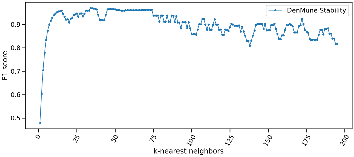
The Stability
The algorithm is only single-parameter, even more it not sensitive to changes in that parameter, k. You may guess that from the following chart yourself. This is of greate benfit for you as a data exploration analyst. You can simply explore the dataset using an arbitrary k. Being Non-senstive to changes in k, make it robust and stable.
Reveal the propagation
one of the top performing feature in this algorithm is enabling you to watch how your clusters propagate to construct the final output clusters. just use the parameter ‘prop_step’ as in the following example:
dataset = "t7.10k" #
data_path = 'datasets/denmune/chameleon/'

# train file
data_file = data_path + dataset +'.csv'
X_train = pd.read_csv(data_file, sep=',', header=None)


from itertools import chain

# Denmune's Paramaters
knn = 39 # number of k-nearest neighbor, the only parameter required by the algorithm

# create list of differnt snapshots of the propagation
snapshots = chain(range(2,5), range(5,50,10), range(50, 100, 25), range(100,500,100), range(500,2000, 250), range(1000,5500, 500))

from IPython.display import clear_output
for snapshot in snapshots:
    print ("itration", snapshot )
    clear_output(wait=True)
    dm = DenMune(train_data=X_train, k_nearest=knn, rgn_tsne=False, prop_step=snapshot)
    labels, validity = dm.fit_predict(show_analyzer=False, show_noise=False)
How to Run and Test
Interact with the algorithm

This notebook allows you interact with the algorithm in many asspects:
you can choose which dataset to cluster (among 4 chameleon datasets)
you can decide which number of k-nearest neighbor to use
show noise on/off; thus you can invesitigate noise detected by the algorithm
show analyzer on/off
Repo2Docker Binder
Launch Examples in Repo2Docker Binder
Simply use our repo2docker offered by mybinder.org, which encapsulate the algorithm and all required data in one virtual machine instance. All jupter notebooks examples found in this repository will be also available to you in action to practice in this respo2docer. Thanks mybinder.org, you made it possible!
Kaggle workspace
Launch each Example in Kaggle workspace
If you are a kaggler like me, then Kaggle, the best workspace where data scientist meet, should fit you to test the algorithm with great experince.
Dataset
Kaggle URL
When less means more - kaggle
Non-groundtruth datasets - kaggle
2D Shape datasets - kaggle
MNIST dataset kaggle
Iris dataset kaggle
Training MNIST to get 97%
Noise detection - kaggle
Validation - kaggle
The beauty of propagation - kaggle
The beauty of propagation part2 - kaggle
Snapshots of propagation -kaggle
Scalability kaggle
Stability - kaggle
k-nearest-evolution - kaggle
Google Research, CoLab
Launch each Example in Google Research, CoLab
Need to test examples one by one, then here another option. Use colab offered by google research to test each example individually.
Here is a list of Google CoLab URL to use the algorithm interactively
Dataset
CoLab URL
How to use it - colab
Chameleon datasets - colab
2D Shape datasets - colab
MNIST dataset - colab
iris dataset - colab
Get 97% by training MNIST dataset - colab
Non-groundtruth datasets - colab
Noise detection - colab
validation - colab
How it propagates - colab
Snapshots of propagation - colab
Scalability - colab
Stability vs number of nearest neighbors - colab
k-nearest-evolution - colab
How to cite
If you have used this codebase in a scientific publication and wish to cite it, please use the Journal of Pattern Recognition article
Mohamed Abbas McInnes, Adel El-Zoghaby, Amin Ahoukry, *DenMune: Density peak based clustering using mutual nearest neighbors*
In: Journal of Pattern Recognition, Elsevier, volume 109, number 107589.
January 2021
@article{ABBAS2021107589,
title = {DenMune: Density peak based clustering using mutual nearest neighbors},
journal = {Pattern Recognition},
volume = {109},
pages = {107589},
year = {2021},
issn = {0031-3203},
doi = {https://doi.org/10.1016/j.patcog.2020.107589},
url = {https://www.sciencedirect.com/science/article/pii/S0031320320303927},
author = {Mohamed Abbas and Adel El-Zoghabi and Amin Shoukry},
keywords = {Clustering, Mutual neighbors, Dimensionality reduction, Arbitrary shapes, Pattern recognition, Nearest neighbors, Density peak},
abstract = {Many clustering algorithms fail when clusters are of arbitrary shapes, of varying densities, or the data classes are unbalanced and close to each other, even in two dimensions. A novel clustering algorithm “DenMune” is presented to meet this challenge. It is based on identifying dense regions using mutual nearest neighborhoods of size K, where K is the only parameter required from the user, besides obeying the mutual nearest neighbor consistency principle. The algorithm is stable for a wide range of values of K. Moreover, it is able to automatically detect and remove noise from the clustering process as well as detecting the target clusters. It produces robust results on various low and high dimensional datasets relative to several known state of the art clustering algorithms.}
}
Licensing
The DenMune algorithm is 3-clause BSD licensed. Enjoy.
Task List
☒ Update Github with the DenMune sourcode
☒ create repo2docker repository
☒ Create pip Package
☒ create CoLab shared examples
☒ create documentation
☒ create Kaggle shared examples
☐ create conda package